Advanced Temporal Modeling in Foreign Exchange Markets

Image by Google's Nano Banana Pro

Check out Aurum AI on the MQL5 Marketplace

The global financial landscape has undergone a seismic shift, transitioning from human-intermediated floor trading to high-frequency, algorithmic environments that operate at microsecond latencies. This evolution has rendered traditional econometric frameworks, which are primarily rooted in linear assumptions and the Efficient Market Hypothesis (EMH), increasingly inadequate for capturing the non-linear, non-stationary, and high-noise characteristics of modern asset pricing. In this complex arena, deep learning (DL) has emerged as the dominant paradigm, offering architectures capable of uncovering latent structures within massive, heterogeneous datasets. Among these, Long Short-Term Memory (LSTM) networks have risen to prominence as the quintessential tool for modeling temporal dependencies in sequential data, such as exchange rates and commodity prices like gold (XAUUSD).

The surge in market interest is reflected in worldwide search trends, where the term "AI forex trading" reached an all-time historical peak in late 2025, closely followed by "AI trading bots". This trend indicates a growing professional and retail demand for sophisticated, automated systems that can navigate the "complexity arms race" of modern markets. Unlike traditional technical analysis, which relies on hand-crafted indicators and rigid rules, deep learning models like the Aurum system allow the model to discover patterns directly from historical data, adapting to changing market regimes and capturing complex relationships that are invisible to the naked eye.

The Mathematical Mechanics of Gated Information Flow in Recurrent Neural Networks

Financial Forecasting and LSTM Architecture

The primary challenge in financial forecasting is the modeling of long-term temporal dependencies. Exchange rates are not independent and identically distributed (i.i.d.) variables; they are sequences where the current state is deeply influenced by historical context. Standard Recurrent Neural Networks (RNNs) were initially designed to process such sequences, but they are fundamentally limited by the vanishing gradient problem. As gradients are backpropagated through time, the repeated multiplication of small values in the activation function derivatives causes the gradient to decay exponentially, effectively preventing the network from learning dependencies beyond a few time steps.

The Long Short-Term Memory (LSTM) architecture, introduced by Hochreiter and Schmidhuber, resolves this issue through the implementation of a memory cell and a sophisticated gating mechanism. The memory cell acts as a "conveyor belt" or cell state ($C_t$), allowing information to persist across many time steps with minimal modification. This preservation of state is regulated by three primary gates: the forget gate, the input gate, and the output gate.

The Forget Gate and Information Persistence

The forget gate ($f_t$) determines which information from the previous cell state ($C_{t-1}$) is no longer relevant for the current prediction task. This decision is modeled by a sigmoid function:

$$f_t = \sigma(W_f \cdot [h_{t-1}, x_t] + b_f)$$

In financial terms, this might correspond to discarding noise from a stale trading session while retaining the broader multi-day trend. A value of 0 indicates "completely forget," while 1 indicates "completely keep".

The Input Gate and State Update

The input gate ($i_t$) identifies which new information is worth storing in the cell state. This involves a two-step process: a sigmoid layer decides which values to update, and a hyperbolic tangent (tanh) layer creates a vector of new candidate values, $\tilde{C}_t$:

$$i_t = \sigma(W_i \cdot [h_{t-1}, x_t] + b_i)$$

$$\tilde{C}_t = \tanh(W_C \cdot [h_{t-1}, x_t] + b_C)$$

The cell state is then updated through an additive process, which is the mathematical key to preventing gradient collapse:

$$C_t = f_t \cdot C_{t-1} + i_t \cdot \tilde{C}_t$$

The Output Gate and Hidden State Generation

Finally, the output gate ($o_t$) determines what part of the current cell state will be passed to the hidden state ($h_t$), which serves as the network's output for the current step and the input for the next:

$$o_t = \sigma(W_o \cdot [h_{t-1}, x_t] + b_o)$$

$$h_t = o_t \cdot \tanh(C_t)$$

This hidden state represents the "short-term memory" of the network, while the cell state represents its "long-term memory".

Advanced Feature Engineering: Statistical Regime Detection and Volatility Estimation

Raw OHLCV data is generally insufficient for deep learning models to achieve high precision in the noisy Forex environment. Professional-grade systems like Aurum utilize an engineered feature vector—in this case, 51 distinct features—organized into categories that capture different aspects of market behavior.

Statistical Regime Detection via Hurst Exponent and Approximate Entropy

Detecting market regimes—whether the market is trending, mean-reverting, or random—is critical for selecting the appropriate trading strategy. The Hurst Exponent ($H$) is a statistical measure of long-term memory in a time series.

$$H < 0.5 \implies \text{Mean-reverting (anti-persistent) series}$$

$$H = 0.5 \implies \text{Geometric random walk (Brownian motion)}$$

$$H > 0.5 \implies \text{Trending (persistent) series}$$

In the Aurum system, the Hurst Exponent is calculated to measure persistence. If $H > 0.5$, the model identifies a trending regime where past movements are likely to continue. Conversely, Approximate Entropy (ApEn) is used to quantify the amount of regularity and the unpredictability of price fluctuations. A low ApEn value indicates a highly predictable, repetitive pattern, while a higher value suggests a less predictable, complex process. This allows the model to differentiate between "clean" trends and "noisy" consolidation phases.

Multi-Estimator Volatility Analysis

Volatility is not a monolithic metric. Standard deviation (close-to-close) often fails to capture intraday price spikes and overnight gaps. Systems like Aurum implement advanced estimators to gain a more nuanced view of market risk.

Professional trading systems employ multiple volatility estimators to capture different market dynamics. The Parkinson estimator uses only High and Low prices to capture intraday range dynamics. The Garman-Klass estimator incorporates Open, High, Low, and Close data, assuming zero drift, making it more efficient than simple close-to-close calculations. The Rogers-Satchell estimator also uses OHLC data but is specifically designed for non-zero drift conditions, making it effective in trending markets. Finally, the Yang-Zhang estimator combines all OHLC data plus gap analysis, providing minimum error by handling both drift and opening jumps—making it particularly valuable for assets like gold that experience significant overnight volatility.

The Yang-Zhang estimator is particularly valuable for XAUUSD trading because it combines overnight volatility (close-to-open) with a weighted average of Rogers-Satchell and open-to-close volatility, making it 14 times more efficient than standard historical volatility.

The Aurum Implementation: A Technical Deep Dive into XAUUSD Modeling

The Aurum system, developed by Auron Automations, provides a real-world case study of these theories in practice. It operates on the H1 (hourly) timeframe for Gold (XAUUSD), processing a 30-bar lookback window across 51 engineered features.

Dual Neural Network Architecture

Aurum employs a hybrid LSTM-CNN architecture to capture both temporal and spatial patterns. This fusion allows the system to understand the "rhythm" of price movement through the LSTM layers and the "structure" of market microstructure through Convolutional Neural Networks (CNN).

def build_model(self):
   inputs = Input(shape=(30, 51), name='input')
   
   # LSTM Branch - Temporal patterns
   lstm_out = LSTM(units=128, dropout=0.2)(inputs)
   
   # CNN Branch - Spatial patterns  
   cnn_out = Conv1D(filters=128, kernel_size=3, activation='relu')(inputs)
   cnn_out = GlobalMaxPooling1D()(cnn_out)
   
   # Fusion Layer
   fused = Concatenate()([lstm_out, cnn_out])
   fused = Dense(64, activation='relu')(fused)
   fused = Dropout(0.2)(fused)
   
   outputs = Dense(1, activation='linear')(fused)
   
   return Model(inputs=inputs, outputs=outputs)

This hybrid approach is supported by empirical findings suggesting that CNNs excel at detecting localized temporal patterns—such as sudden price spikes or momentum shifts—while LSTMs maintain the long-term context.

Training and Validation: Avoiding Overfitting

One of the most significant risks in financial deep learning is overfitting to historical noise. Aurum addresses this through "gap validation" methodology and the application of early stopping. The training results for the Aurum model show a clear convergence of training and validation loss over 70 epochs. The fact that validation loss closely tracks training loss indicates that no significant overfitting was detected, a critical requirement for out-of-sample performance.

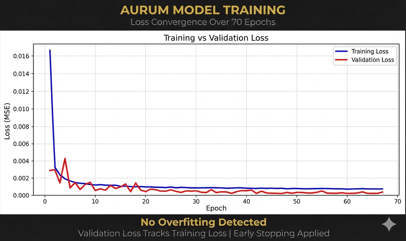
Figure 1: Training and validation loss convergence over 70 epochs, demonstrating no significant overfitting in the Aurum model.

Metric Aurum Model Performance Value R-Squared (R²) 0.7640 Mean Absolute Percentage Error (MAPE) 5.36% Root Mean Squared Error (RMSE) 0.0186 Mean Absolute Error (MAE) 0.0144

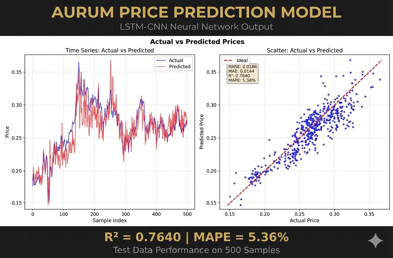
Figure 2: Price prediction scatter plot demonstrating strong linear relationship between actual and predicted prices across 500 samples, with the model effectively capturing volatility and trend shifts in the gold market.

The price prediction scatter plot demonstrates a strong linear relationship between actual and predicted prices across 500 samples, with the model effectively capturing the volatility and trend shifts inherent in the gold market.

Python Implementation Pipeline: From Data Preprocessing to Sequence Modeling

Building a robust LSTM pipeline in Python requires careful attention to data normalization and sequence structuring.

Data Preparation and Scaling

Financial time series are typically non-stationary, meaning their mean and variance change over time. Before feeding data into an LSTM, it must be normalized to a consistent range, typically [0, 1] or [-1, 1], using tools like MinMaxScaler.

from sklearn.preprocessing import MinMaxScaler

# Normalize both test and train data with respect to training data
scaler = MinMaxScaler()
train_data_scaled = scaler.fit_transform(train_data.reshape(-1, 1))
test_data_scaled = scaler.transform(test_data.reshape(-1, 1))

Crucially, the scaler should be fit only on the training data to prevent "data leakage," where information from the future (the test set) influences the training process.

Sequence Generation and Batching

LSTMs require input data in a 3D tensor format: [batch_size, time_steps, features]. For a system like Aurum, which uses a 30-bar lookback, the input data must be reshaped accordingly.

def create_sequences(data, n_steps):
   X, y = [], []
   for i in range(len(data)):
       end_ix = i + n_steps
       if end_ix > len(data) - 1:
           break
       seq_x, seq_y = data[i:end_ix], data[end_ix]
       X.append(seq_x)
       y.append(seq_y)
   return np.array(X), np.array(y)

n_steps = 30
X_train, y_train = create_sequences(train_data_scaled, n_steps)

This "sliding window" approach allows the model to learn how a specific sequence of 30 bars relates to the price of the 31st bar.

Deployment and Real-Time Inference: Integrating Python with MetaTrader 5

The final frontier of AI trading is the deployment of these complex models into real-time execution platforms. Aurum uses the Open Neural Network Exchange (ONNX) format to bridge the gap between Python (training) and MQL5 (execution).

The ONNX Export Logic

Because TensorFlow or PyTorch models cannot run directly inside the MetaTrader 5 terminal, they must be converted to ONNX, an open-standard format for machine learning models.

import torch.onnx

def export_onnx(model, output_path):
   # Export with dynamic batch size for flexible inference
   torch.onnx.export(
       model,
       torch.randn(1, 30, 51),
       output_path,
       input_names=['input'],
       output_names=['output'],
       opset_version=14,
       dynamic_axes={'input': {0: 'batch'}, 'output': {0: 'batch'}}
   )

Expert Advisor (EA) Integration in MQL5

The MetaTrader 5 terminal provides an ONNX API that allows the Expert Advisor to load the model as a resource and run inference on every new tick or bar.

#resource "\\Models\\aurum_lstm.onnx" as uchar PriceModelBuffer[]

int OnInit()
{
  // Create the ONNX model handle from the embedded buffer
  g_price_model = OnnxCreateFromBuffer(PriceModelBuffer, ONNX_DEFAULT);
  
  // Set the input shape to match the Python training configuration
  ulong input_shape[] = {1, 30, 51};
  OnnxSetInputShape(g_price_model, 0, input_shape);
  
  return INIT_SUCCEEDED;
}

To optimize performance, Aurum implements a feature caching system. Instead of recomputing 51 features for all 30 bars on every tick (an $O(30 \times 51)$ operation), it uses a circular buffer to update only the newest bar, achieving $O(51)$ efficiency.

Real-Life Results and Comparative Benchmarks in Modern Research

The effectiveness of LSTMs and their variants is well-documented across recent academic and industry studies. While LSTMs are powerful, they are often compared against other architectures to find the optimal balance of accuracy and computational efficiency.

Comparative Performance: LSTM vs. GRU vs. ARIMA

In a 2025 study of foreign exchange rate predictions (USD, EUR, GBP against THB), Gate Recurrent Units (GRU) and LSTMs demonstrated superior accuracy over traditional models and even complex attention-based models like the Temporal Fusion Transformer (TFT).

This research suggests that while transformers like TFT are powerful for long-horizon forecasting, their complexity can lead to poor performance on high-frequency financial data that lacks sufficient time-varying features. LSTMs and GRUs provide a more robust middle ground for capture-and-predict tasks in liquid markets.

Case Study: Gold (XAUUSD) Prediction Accuracy

Research conducted on individual stocks and commodities like gold indicates that LSTMs excel in stable, high-liquidity sectors. A multi-year dataset study demonstrated an R² > 0.87 for stocks in power generation and fertilizers, though gold often presents a lower R² due to its sensitivity to sudden geopolitical shifts and the "Safe Haven" effect.

One critical scientific finding from session-based studies of gold is that predicting the exact percentage return is extremely difficult, often resulting in negative R² scores for regression models. However, classification tasks—predicting whether the price will go up or down (directional movement)—yield far better results. For example, an XGBoost champion model achieved 54% directional accuracy, which was sufficient to generate a profitable trading edge after commissions.

Risk Management: The Final Component of Algorithmic Success

No neural network, regardless of its architectural complexity, can succeed without a robust risk management framework. The non-stationary nature of markets means that patterns discovered during training may disappear or invert during a regime shift.

Dynamic Position Sizing and ATR-Based Controls

Aurum utilizes Average True Range (ATR) to set dynamic stop-loss (SL) and take-profit (TP) levels.

• •

  Stop Loss: Set at 3x ATR to allow for market noise while protecting against structural breakdowns.

• •

  Take Profit: Set at 6x ATR, maintaining a 1:2 risk-to-reward ratio.

This approach ensures that the system does not rely on dangerous strategies like martingale, grid, or averaging, which are common in failed algorithmic systems.

Sentiment Analysis and Multi-Modal Fusion

The most advanced trading systems are moving toward multi-modal fusion, where numerical price data is combined with textual sentiment from news reports and social media. Models like FinBERT, a pre-trained BERT model specialized for the financial domain, can classify sentiment with over 86% accuracy. By integrating sentiment as a feature, an LSTM can "understand" whether a price spike is backed by fundamental news or is merely a technical correction.

Operational Summary and Future Outlook

The technical deep dive into LSTM networks for Forex reveals a discipline at the intersection of mathematical rigor and high-speed engineering. The ability of LSTMs to solve the vanishing gradient problem through their unique gating architecture remains the foundation for temporal modeling in finance. However, as the Aurum implementation demonstrates, the highest-performing systems are those that weave together these neural networks with sophisticated feature engineering—including Hurst Exponents and Yang-Zhang volatility—and deploy them via optimized runtimes like ONNX.

The transition toward "Large Investment Models" and multi-agent systems suggests a future where specialized LLM agents debate and refine strategies, mitigating individual model biases and improving overall system robustness. While the market continues to be a high-noise environment, the combination of LSTM's temporal memory and CNN's spatial pattern extraction provides a mathematically sound basis for identifying the subtle edges that traditional analysis overlooks. For the quantitative trader, success is not a function of finding a "perfect" model, but of building a stable, adaptive pipeline that respects the non-stationarity and inherent risk of the global financial system.